Beyond the Grid: Mastering Urban Complexity with Graph Neural Networks

Have you ever wondered why a minor accident on a quiet side street can eventually gridlock a major highway miles away? It happens because our cities aren’t just collections of isolated roads; they are complex, living webs where everything is connected to everything else.

To make sense of this complexity, we need technology that doesn’t just look at data points in isolation, but understands the relationships between them. To “see” the intricate geometry of a city, enter Graph Neural Networks (GNNs)—models designed specifically to master these connections. But what exactly is a “graph” in the world of AI? How do these models manage to pass information between different parts of the network? And how can they help transportation?

In this article, we will guide you through the fundamentals of GNNs, how they work, some of their applications in transport, and the challenges that lie ahead.

1. Thinking in Graphs

At its simplest, a Graph is a way of modeling the physical world as it actually exists: connected and relational. GNNs are the AI engines built to operate on this reality. Unlike standard models that treat data as isolated lists, GNNs have a “built-in intuition” (technically known as inductive bias) that assumes the relationships between data points are as important as the data itself.

To understand how this works, we will first identify the raw ingredients of a graph (nodes and edges), then detail the engine that powers them (message passing), and finally explain why GNNs outperform traditional methods when dealing with complex network structures.

1.1. The ingredients: nodes and edges

In a standard Excel spreadsheet, every row is independent. But in transportation, nothing exists in a vacuum. Think of a subway map. The map doesn’t show you the exact geographical coordinates of every station; instead, it shows you the topology: how Station A connects to Station B. To capture this reality, we use a Graph.

A graph consists of two simple ingredients: Nodes (the “things”) and Edges (the “connections”). There is no single “correct” way to draw a graph; it depends entirely on the problem you want to solve. For example, if you are analyzing traffic congestion, nodes might be intersections and edges the roads connecting them. If you shift your focus to urban mobility, those nodes might become “Points of Interest” (like schools or business districts) with edges representing the movement of people between them. On a global scale, nodes could be entire countries, with edges indicating trade agreements. The flexibility of the graph allows us to model almost any system where relationships matter more than raw data points.

With the edges in place, we can go a step further. Not all connections are created equal; some are stronger or more important than others. To capture this, we assign weights to the edges. Mathematically, we organize these weights into an adjacency matrix, which is essentially a grid or lookup table where a positive number represents the strength of a connection, and a zero means no connection exists.

Determining these weights depends heavily on the context. In a road network, for instance, weights are often assigned inversely to the distance. If two intersections are very close, they have a “strong” connection (a high weight) because a traffic jam at one will almost certainly impact the other. Conversely, in a logistics network, physical distance might matter less than economic ties. Two major capitals might be physically far apart, yet have a very high connection weight due to the intense volume of trade flowing between them. Furthermore, a network isn’t limited to just one set of weights. We can have multiple adjacency matrices for the same graph where one tracks physical distance, another tracks speed limits, and a third tracks truck volume. This allows us to create a rich, multi-layered picture of the transportation system.

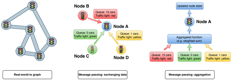
Figure 1: The inner workings of a Graph Neural Network for traffic prediction. Panel 1 shows how a physical road network is transformed into a graph, where intersections become “nodes” and roads become “edges.” Panel 2 demonstrates “message passing,” where neighboring intersections (Nodes B, C, D) share real-time data, such as queue length and traffic light status, with a central node (Node A). Panel 3 illustrates that the incoming messages are processed through an “Aggregation Function” to update Node A’s state.

1.2. The mechanism: message passing

Now that we have built our graph with nodes, edges, and weights, the question remains: how does the model actually “learn” from this structure? This brings us to the heartbeat of a GNN, a process known as Message Passing. You can think of this as a massive, simultaneous conversation happening across the entire network. In a traditional model, a data point is isolated, but in a GNN, every node actively queries its neighbors to better understand its own situation.

As shown in the figure 1, imagine intersections trying to predict their traffic for the next ten minutes. They first “listen” to the messages sent by their neighbors, which contain crucial information about upstream congestion or accidents. The node collects all these incoming signals and aggregates them into a summary weighted by the adjacency matrix. This ensures that the node prioritizes signals from important neighbors, such as giving more weight to closer intersections if the matrix is based on distance. Finally, it combines this external wisdom with its own internal data to update its state. By repeating this process in multiple rounds or “layers”, a node can eventually gain awareness of conditions miles away, effectively allowing local interactions to solve global network problems.

But where does the “Neural” part come in? Neural networks are embedded directly into this process to act as translators. Before a message is sent, the network transforms the raw signals—such as a simple report of an accident—into a more information-rich space. This ensures that when a node receives messages from its neighbors, it isn’t just getting basic statistics; it is receiving context and patterns encoded in a language that the model can deeply understand and process.

1.3. The differentiator: why not standard AI?

We already have incredible AI that can drive cars and recognize faces. Why do we need a special “Graph” neural network? Why can’t we just take a snapshot of the city and feed it into standard image-recognition models?

The answer lies in the geometry. Standard AI (specifically Convolutional Neural Networks, or CNNs) is built for grids. Think of a digital image: it is a perfect checkerboard of pixels where every single point is neatly arranged in rows and columns, and every pixel has exactly the same number of neighbors. This rigid structure is what mathematicians call “Euclidean” space.

But a city is not a checkerboard; it is a messy, irregular web. Unlike a pixel grid, transportation networks are full of inconsistencies. One intersection might connect to five different roads, while another connects to just two. Similarly, two sensors might be miles apart physically yet inextricably linked by a fast highway, while two others sit adjacent to each other but are separated by a river. If you try to force this complex, “non-Euclidean” reality into a rigid grid just to satisfy standard AI, you lose the most valuable information: the topology. It is like trying to flatten a globe onto a piece of paper and inevitably distort the map. GNNs are the differentiator because they don’t demand a grid. They are designed to be flexible, respecting the unique, irregular shape of the transportation network and processing the data exactly as it exists in the real world.

2. Applications in Practice

Consider travel time estimation. Traditional models treated roads independently, blind to how congestion bleeds between routes. ConSTGAT, deployed within Baidu Maps, instead looks at the parallel routes absorbing overflow, the on-ramps feeding volume, and the bottlenecks that have not yet materialized. By combining a graph attention network with a temporal component, it captures both the spatial conversation between roads and its duration. The result is not just a prediction, but an awareness of the network as a system. [1]

Network-wide speed forecasting follows the same logic at a larger scale. On a single corridor, a time-series model might suffice. But across hundreds of sensors, a slowdown propagates quietly to feeder roads kilometers away. DCRNN treats this as a diffusion process, encoding the network into a bidirectional random walk that learns to propagate spatial and temporal dependencies simultaneously. It does not wait for congestion to arrive; it anticipates its path. [2]

In public transport, the challenge intensifies. A bus moves within general traffic; when it is stuck, it alters passenger loads at downstream stops, shifting crowding across the entire route. TMS-GNN embeds real-time traffic conditions directly into the graph of bus stops and routes. Its multi-task framework predicts both traffic states and passenger flows, capturing how delays propagate. [3] For agencies, this means moving beyond static schedules to dynamic understanding: where crowding will occur, how to adjust dispatching, what information passengers need.

In strategic planning, the question is not whether a new bike-share station will be used, but how it will rewire usage across the entire system. The GNN developed for Toronto and Vancouver treats station-to-station trips as a graph and simulates “what-if” scenarios before any infrastructure is built. By learning latent dependencies through graph convolutional layers, it predicts demand at the new node and the resulting shifts at every connected node. [4] Planners gain the ability to see second-order effects.

This logic extends beyond mobility into energy. In dynamic smart charging, where vehicles arrive continuously and grid capacity is finite, power allocation is a coordination problem across vehicles, stations, and time. GNN-DT (Graph Neural Network enhanced Decision Transformer), developed at TU Delft, treats each vehicle and station as nodes in a bipartite graph, with edges representing eligibility and temporal dependencies. Through message passing, it learns the structure of these interactions, anticipates conflicts, adapts in real time, and optimizes collectively. The graph is not a map of the system—it is the system itself. [5]

Across every application, the pattern is the same. Those who succeed with GNNs recognize that their problem was never about isolated sensors, independent roads, or standalone stations. It was always about the relationships between them.

3. From Theory to Practice: A Guide for Implementation

Successfully translating GNN research into operational systems requires moving beyond the algorithms to focus on design strategy. For practitioners looking to deploy these models, we recommend focusing on the following key pillars.

3.1. Define the right graph

Defining the graph is the foundational step, often more critical than the model architecture itself. We advise practitioners to look beyond simple physical adjacency and focus on the specific relationships that drive the system. Furthermore, consider whether the problem requires a static structure or a dynamic one that adapts to incidents in real-time. The graph is your primary vehicle for encoding domain knowledge; if a single perspective is insufficient, do not hesitate to combine them.  For instance, the DG4b method developed at TU Delft effectively fuses two distinct graphs—one representing static road infrastructure and another capturing dynamic cycling routes—to significantly improve bicycle travel time estimation.[6]

3.2. Keep the architecture focused

When designing the neural network, simpler is often better. Driven by the message passing mechanism, each GNN layer expands a node’s “receptive field” by exactly one step.  While a 2-layer network effectively captures the context of neighbors-of-neighbors, adding too many layers causes a phenomenon known as over-smoothing. In this state, unique local details are washed out because every node eventually aggregates information from the entire graph, making their representations indistinguishable. For most transportation networks, we recommend limiting the depth to two to four layers. This captures the necessary spatial dependencies (the immediate neighborhood and its neighbors) while preserving the distinct, local signals of each node.

3.3. Plan for scale and speed

Moving from a test dataset to a city-wide network with thousands of segments changes the computational game. To efficiently manage this scale, we suggest techniques like graph sampling or training on subgraphs, which allow the model to learn representative patterns without processing the entire network at every step. For real-time inference, where predictions must be generated in seconds, consider knowledge distillation. This approach allows you to train a complex, high-accuracy teacher model and then “compress” its knowledge into a leaner student model suitable for deployment. This engineering mindset, exemplified by systems like Baidu’s ConSTGAT, is essential for bridging the gap between academic prototyping and real-world latency requirements.

4. Conclusion

The transition to GNNs represents more than just an algorithmic upgrade; it marks a fundamental shift in how we model the physical world. We are moving from viewing transportation as a collection of isolated data points to understanding it as a complex system defined by its connections.

Standard AI methods, built for rigid, grid-like structures, often fail to capture the irregular, non-Euclidean geometry of real cities.  GNNs bridge this gap by embedding the network’s topology directly into the learning process, allowing the model to see the structure of the transportation network as it exists in reality.

However, complexity should not be the default. For practitioners, the adoption of GNNs should follow a hierarchy of necessity. If the problem is local and interactions are weak, classical methods remain robust and efficient. But when network effects predominate—when the state of a node is inextricably linked to its neighbors—incorporating spatial structure via GNNs becomes essential. As we move from theory to practice, success will not be determined by raw computing power, but by the strategic design of graphs that balance rich domain representation with scalable engineering. Yet, the potential payoff is immense. By successfully modeling the “living web” of our cities, GNNs offer the promise of transportation systems that are not just reactive, but truly intelligent and predictive.

---

[1] See Xiaomin Fang et al., ConSTGAT: Contextual Spatial-Temporal Graph Attention Network for Travel Time Estimation at Baidu Maps (2020), in KDD ’20: Proceedings of the 26th ACM SIGKDD International Conference on Knowledge Discovery & Data Mining, pp. 2697-2705.

[2] See Yaguang Li et al., Diffusion Convolutional Recurrent Neural Network: Data-Driven Traffic Forecasting (2017), published as a conference paper at ICLR 2018.

[3] See Asiye Baghbani et al., TMS-GNN: Traffic-Aware Multistep Graph Neural Network for Bus Passenger Flow Prediction (2025), in Transportation Research Part C: Emerging Technologies, Volume 174, May 2025, 105107.

[4] See Ghazaleh Mohseni et al., Bike-Sharing Ridership Prediction for Network Expansion Using Graph Neural Networks, in Transportation Research Part A: Policy and Practice, Volume 203, January 2026, 104701.

[5] See Stavros Orfanoudakis et al., A Graph Neural Network Enhanced Decision Transformer for Efficient Optimization in Dynamic Smart Charging Environments in Energy and AI, Volume 23, January 2026, 100679.

[6] See Ting Gao et al., Bicycle Travel Time Estimation via Dual Graph-Based Neural Networks in IEEE Transactions on Intelligent Transportation Systems, Volume 27, Issue 1.