Time-Series Modeling for Mobility: Why LSTMs Still Matter

Modern mobility systems generate a constant stream of data—from link speeds and dwell times to passenger flows and signal states. Turning these signals into reliable short-term forecasts is essential for operations, customer information, and network management. While classical time-series models remain strong baselines, today’s complex and dynamic networks increasingly benefit from methods that can remember what parts of recent history still matter. This article introduces Long Short-Term Memory (LSTM) models in a practical, transport-focused way, showing where they add value, how they work, and what to consider when deploying them.

1. From Classical Forecasting to Sequence Learning in Mobility

Mobility runs on clocks and counts. Sensors report minute-by-minute data such as link speeds and volumes. Forecasts turn this streaming data into operating decisions and into the real-time estimates travellers see on platform displays and roadside signs. The central questions are usually short-horizon and practical—for example, whether a corridor will slow in the next quarter hour. Because incidents and weather often disrupt routine, we need models that preserve the parts of recent history that still matter.

Classical methods have long provided dependable answers. When patterns are regular, exponential smoothing often suffices. For linear and stationary data, ARIMA (or its seasonal extension) is a natural choice. When dynamics are mechanistic and near-linear, state-space models with Kalman filtering come to the fore (Box et al. 2015; Hyndman and Athanasopoulos 2021). These methods remain transparent, data-efficient, and frequently “good enough” in stable regimes where seasonality and autocorrelation behave themselves.

The difficulty is that modern urban networks are rarely that tidy. As fleets and infrastructure have become densely instrumented, relationships have grown more entangled. In response, practitioners first turned to machine-learning methods that could absorb more inputs and interactions. Regularized regressions and gradient-boosted trees can handle dozens of lags, calendar and weather features, and event indicators, and often outperform hand-tuned formulas. Yet they still treat time as a fixed window chosen in advance, which makes long-range and context-dependent effects easy to miss. That limitation pushed the field toward deep sequence models. Early recurrent networks attempted to learn temporal dependence directly but struggled to carry information over long spans as gradients faded. Long Short-Term Memory (LSTM) networks address this by adding gates that learn what to retain, what to overwrite, and what to reveal from an internal memory (Hochreiter and Schmidhuber 1997).

Transport forecasting is, at heart, the art of carrying forward a compact summary of recent history. In stable regimes, classical models (exponential smoothing, ARIMA, and state-space/Kalman filters) remain reliable baselines because they capture level, trend, and seasonality with admirable economy (Box et al. 2015; Hyndman and Athanasopoulos 2021). Many mobility signals are not so obliging: link speeds reflect upstream queues and signal cycles, dwell times respond to crowding and events, and condition-monitoring streams drift for weeks and then jump. In those settings, we want models that learn which parts of the past matter, and for how long. In summary, LSTMs learn which parts of yesterday’s disruption still matter for this morning’s peak, which upstream closure still shapes your link twenty minutes later, and which vibration drift is meaningful rather than noise.

2. A General Technical Overview

In practice, we model traffic as a time series—ordered measurements in which daily and weekly rhythms, along with responses to weather and incidents, often repeat. The objective is to learn these patterns with suitable models or techniques so we can approximate how they evolve under similar conditions. By capturing them, we can both predict near-term conditions and analyze what-if scenarios when inputs change.

This section provides a quick look at the LSTM cell through a traffic-flow example. The appeal is simple: an LSTM can remember the parts of recent history that still matter, and it can forget stale context. Imagine predicting corridor speed a few minutes ahead. Each minute, the input may include the latest link speed, a few upstream speeds, signal phase, weather, and an event flag. Inside the cell, the model maintains two tracks at time t. The hidden state hₜ is a short summary that feeds the next computation. The cell state cₜ is a longer memory that carries context forward. It helps to think of three decisions that occur every minute.

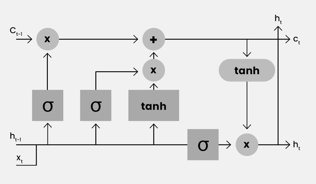
Figure 1: An LSTM cell. The circles show elementwise multiply and add. The boxes are learned layers with σ or tanh.

• Keep. The top track carries the previous memory cₜ₋₁. The left sigmoid (σ) layer produces a keep gate fₜ between zero and one. Multiplying fₜ with cₜ₋₁ controls retention. If detectors report sustained low speeds for several minutes, fₜ typically sits around 0.8–1.0 so the queue context is preserved. When speeds return to typical off-peak values, fₜ moves toward 0.1–0.3 and the old context is cleared.
• Write. The middle tanh block proposes new content gₜ from the latest inputs, such as an upstream slowdown or the onset of rain. A second sigmoid (σ) layer forms an input gate iₜ. The updated memory cₜ is the sum of the kept part fₜ⊙ cₜ₋₁ and the gated proposal iₜ⊙ gₜ. If upstream speed drops by more than 15 km/h within two minutes or an event flag switches on, iₜ is often near 0.7–0.9 so the new situation is written into memory. If speed wiggles by only 1–2 km/h, iₜ stays closer to 0.1–0.3 and the memory barely changes.
• Reveal. The right tanh block transforms the updated memory. A third sigmoid (σ) layer forms an output gate oₜ. The right circle multiplies oₜ with the transformed memory to produce the hidden state hₜ. During a disruption, oₜ tends to expose more of the stored context so the prediction reflects the incident. Once conditions normalize, oₜ reduces exposure and the output returns to routine behaviour.

The numeric ranges above are illustrative. The network learns gate values from data, allowing it to retain sustained effects such as queues while downweighting small fluctuations. The three gates act as smooth switches that decide what to keep, what to write, and what to reveal at each step. Because the cell state carries information forward with controlled updates, important traffic context can persist across many minutes. This design addresses the forgetting that limited early recurrent models (Hochreiter and Schmidhuber 1997).

Usually, a shallow stack works well. For short horizons, one or two LSTM layers are enough. For longer horizons, an encoder and decoder work together: the encoder summarizes recent history, and the decoder predicts the future step by step, conditioned on the encoded history and on its own previous predictions (Qin et al. 2017). Because operations manage risk, predictions are best reported as a distribution with a central estimate and an uncertainty band (Salinas et al. 2020). To curb error buildup in multistep forecasts, teach the decoder to handle its own outputs by gradually mixing them with the true last value during training (Bengio et al. 2015).

3. Where LSTMs Already Add Value

This section presents several representative settings where learned temporal memory has made a practical difference in day-to-day operations. The common thread is the need to carry forward the right information from an evolving context.

3.1. Estimated Arrival Times and Network-Aware Forecasting

Estimated arrival times are central to operations, customer information, and fleet control. The strongest systems combine learned temporal memory with explicit network structure. In one large-scale production system, graph-neural components encode the road network and its current state, while recurrent components capture temporal dynamics. The result is a reduction in arrival-time errors that matter most to travelers and dispatchers. The lesson is clear: temporal memory and spatial structure work best together, and a compact LSTM often supplies the temporal side of that partnership (Derrow-Pinion et al. 2021).

3.2. Short-Horizon Traffic and Corridor Speeds

On a single corridor or a handful of links, an LSTM can capture rush-hour buildup and dissipation with little feature engineering. As the spatial scope grows to dozens or hundreds of sensors, network effects dominate and graph-recurrent hybrids become more persuasive. One influential design models how conditions diffuse over the road network with a graph operator and pairs that with a recurrent predictor that remains familiar to practitioners. The approach has been shown to improve accuracy on real sensor networks while keeping the training routine within reach of transport teams (Li et al. 2018).

3.3. Ridership, Dwell, and Platform Management

Ridership and arrivals follow daily and weekly rhythms but break on holidays and major events. A compact LSTM learns how long recent conditions should matter and turns headways, boardings, and simple event flags into short-term forecasts for dwell times and platform-crowding risk. When spatial effects are important, pairing temporal memory with a network graph improves station- or stop-level flow prediction and reduces the hand-tuning needed in rule-based pipelines. A bus-network study that fused graph structure with an LSTM reported stronger short-horizon passenger-flow forecasts on real operations data—the pattern most transit teams care about (Baghbani et al. 2023).

3.4. Signal Timing and Phase Prediction

Adaptive control benefits from short-horizon forecasts of cycle length and phase splits. An LSTM that ingests high-resolution detector counts and phase states can predict time to green and next-cycle durations several cycles ahead. This supports priority logic and speed advice with fewer manual rules. A small convolutional front end can summarize within-cycle patterns, while the LSTM carries state across cycles. On real intersections, this design achieved accurate cycle and phase predictions from detector data and offers a clear blueprint for deployment (Islam et al. 2022).

4. Practical Considerations for Deployment

This section outlines several practical considerations for using LSTM forecasters in day-to-day operations.

4.1. Data Scope and Coverage

Data frequency should match the decision at hand. For link speeds, headways, and dwell times, a few months of one- to five-minute history usually capture everyday rhythms and common disruptions. For planning horizons, years of daily or weekly data are more appropriate. Timestamps and time zones should follow one standard across all sources—many errors that appear to be modeling failures turn out to be timing mismatches. Missing values require explicit treatment: small gaps can be forward- or backward-filled and flagged so the model does not mistake them for real readings; longer gaps are better handled with model-based imputation that borrows strength from related signals, or by sidelining persistently unreliable sensors for a period.

4.2. Features and Model Scope

A good baseline is usually simple, drawing on a recent window of the target variable, calendar variables, and a small set of weather and event indicators. Where a link is influenced by upstream segments, those signals should be included explicitly. If network effects dominate, a graph-aware model is the more honest choice rather than expecting a plain LSTM to infer topology. In risk-sensitive settings, probabilistic outputs should convey a central estimate together with an uncertainty band rather than a single number.

4.3. Drift and Retraining

Patterns in transport shift as construction, detours, service updates, and seasons reshape behavior. Continuous performance monitoring on a rolling window reveals change early, and retraining should be triggered when peak-period error rises or when prediction-interval coverage slips. Mild drift often responds to fine-tuning from the latest checkpoint and to updates to scalers, holiday calendars, and event markers. Clear structural breaks call for a clean retrain on updated history. Maintaining a brief changelog for data and service updates helps keep performance shifts traceable.

4.4. Uncertainty that travels through the pipeline

When a forecast feeds a downstream decision, its uncertainty should travel with it. For example, when link-speed forecasts drive predicted arrivals at stops, propagate the distribution through the mapping step so the uncertainty that matters to the dispatcher appears as an arrival-time band rather than a speed error bar. Modern recurrent forecasters support this style of end-to-end probabilistic modeling and have been shown to produce well-calibrated predictions in practice.

5. Conclusion

Forecasting in mobility is a practical discipline that turns data into actions. Classical methods remain dependable when patterns are stable, while LSTMs help when interactions are strong and the influence of recent history depends on context. The most effective systems combine complementary strengths: LSTMs for temporal memory, graph layers for how conditions spread through a network, and simple decompositions for structural components. Probabilistic forecasts fit daily operations because teams manage risk rather than averages. Confidence grows through careful evaluation and monitoring, with clear test windows, honest comparisons to baselines, and visible uncertainty. A sensible path is to begin with the simplest approach that serves the decision, add learned temporal memory when needed, introduce spatial structure when network effects dominate, and let real deployments guide the next improvement.

---

References

Baghbani, Asiye, Nizar Bouguila, and Zachary Patterson (2023). Short-Term Passenger Flow Prediction Using a Bus Network Graph Convolutional Long Short-Term Memory Neural Network Model. Transportation Research Record 2677 (2): 1331–40.

Bengio, Samy, Oriol Vinyals, Navdeep Jaitly, and Noam Shazeer (2015). Scheduled Sampling for Sequence Prediction with Recurrent Neural Networks. Advances in Neural Information Processing Systems 28.

Box, George EP, Gwilym M Jenkins, Gregory C Reinsel, and Greta M Ljung (2015). Time Series Analysis: Forecasting and Control. John Wiley & Sons.

Derrow-Pinion, Austin, Jennifer She, David Wong, et al. (2021). Eta Prediction with Graph Neural Networks in Google Maps. Proceedings of the 30th ACM International Conference on Information & Knowledge Management, 3767–76.

Hochreiter, Sepp, and Jürgen Schmidhuber (1997). Long Short-Term Memory. Neural Computation 9 (8): 1735–80.

Hyndman, Rob J., and George Athanasopoulos (2021). Forecasting: Principles and Practice. 3rd ed.

Islam, Zubayer, Mohamed Abdel-Aty, and Nada Mahmoud (2022). Using CNN-LSTM to Predict Signal Phasing and Timing Aided by High-Resolution Detector Data. Transportation Research Part C: Emerging Technologies 141: 103742.

Li, Yaguang, Rose Yu, Cyrus Shahabi, and Yan Liu (2018). Diffusion Convolutional Recurrent Neural Network: Data-Driven Traffic Forecasting. International Conference on Learning Representations.

Qin, Yao, Dongjin Song, Haifeng Cheng, Wei Cheng, Guofei Jiang, and Garrison W Cottrell (2017). A Dual-Stage Attention-Based Recurrent Neural Network for Time Series Prediction. Proceedings of the 26th International Joint Conference on Artificial Intelligence, 2627–33.

Salinas, David, Valentin Flunkert, Jan Gasthaus, and Tim Januschowski (2020). DeepAR: Probabilistic Forecasting with Autoregressive Recurrent Networks. International Journal of Forecasting 36 (3): 1181–91.